Posts
Week-3
Categories: figure
Tags: JCO, survival, Kaplan-Meier, survminer
This week’s topic is a survival figure.
Survival does not mean only survival (the state of continuing to live). Survival figures (mostly showing Kaplan-Meier curves) can be used in any time-to-event data using survival function - S(t).
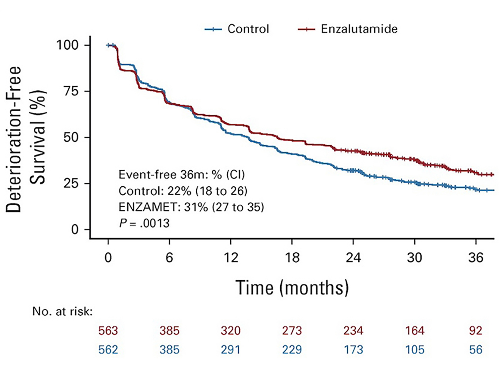
In this RCT, Deterioration-free survival was used for the event which is “physical functioning”.
Any time-to-event data requires two variables for each observation.
- time (time to the event/censor)
- event (event vs. censored)
Fabricating survival data is little bit difficult. simsurv package can be used to simulate survival data,
but I preferred using sliced dataset for each 6-month period for the replication purpose.
It is almost impossible to have exactly same curves, survival percentages, log-rank p value. But similar can be achieved.
Selected article:
Title: Health-Related Quality of Life in Metastatic, Hormone-Sensitive Prostate Cancer: ENZAMET (ANZUP 1304), an International, Randomized Phase III Trial Led by ANZUP
Journal: Journal of Clinical Oncology
Authors: Stockler MR, Martin AJ, Davis ID, et al.
Year: 2021
PMID: 34928708
DOI: 10.1200/JCO.21.00941
The original figure
Import libraries
suppressPackageStartupMessages(library(tidyverse))
suppressPackageStartupMessages(library(fabricatr))
suppressPackageStartupMessages(library(glue))

suppressPackageStartupMessages(library(survival))
suppressPackageStartupMessages(library(survminer))
# suppressPackageStartupMessages(library(simsurv))          # can be used to simulate survival data, but not needed here.

theme_set(theme_light(base_family = "Rubik"))
Prepare fabricated data
n_exp <- c(563, 385, 320, 273, 234, 164, 92, 0)
n_control <- c(562, 385, 291, 229, 173, 105, 56, 0)

fu_one_period_experimental <- vector()
fu_one_period_control <- vector()

for (i in 1:length(n_exp)-1){
  fu_experimental <-  n_exp[i] - n_exp[i + 1]
  fu_control <-  n_control[i] - n_control[i + 1]

  fu_one_period_control[i] <- fu_control
  fu_one_period_experimental[i] <- fu_experimental
}


p_control <- c(.90, .85, .82, .50, .40, .30)
p_exp     <- c(.81, .92, .70, .50, .40, .30)

dataset_experimental_all <- list()
dataset_control_all <- list()

for (i in 1:(length(n_exp)-1)){
set.seed(2022)
dataset_experimental <- fabricate(
  N = fu_one_period_experimental[i],
  fu_time = runif(N, min = 0, max = 6),
  event = draw_binary(prob = p_exp[i], N = N)
) %>%
  as_tibble() %>%
  mutate(event_time = fu_time + 6 * (i - 1),
         group = "experimental")

dataset_experimental_all[[i]] <- dataset_experimental
}
unlist_experimental <-  map_dfr(dataset_experimental_all, bind_rows) %>%
  mutate(event = replace_na(event, 0))


for (i in 1:(length(n_control)-1)){
set.seed(2022)
dataset_control <- fabricate(
  N = fu_one_period_control[i],
  fu_time = runif(N, min = 0, max = 6),
  event = draw_binary(prob = p_control[i], N = N)
) %>%
  as_tibble() %>%
  mutate(event_time = fu_time + 6 * (i - 1),
         group = "control")

dataset_control_all[[i]] <- dataset_control
}
unlist_control <-  map_dfr(dataset_control_all, bind_rows)

combined_dataset <- bind_rows(unlist_experimental, unlist_control) %>%
  select(-fu_time) %>%
  mutate(event_time = round(event_time, 2),
         event = replace_na(event, 0),
         group = fct_relevel(group, "experimental", "control"))
R codes for the figure
model_plot <-  survfit(Surv(event_time, event) ~ group, data = combined_dataset)

summary_surv <- summary (model_plot, times = 36)                             # to add annotation (survival rates) to the figure
surv_diff <- surv_pvalue(model_plot, method = "log-rank")                    # to add annotation (p-value) to the figure
surv_text <-  glue("Event-free 36m: % (CI)
Control: {round(100 * summary_surv$surv[2], 0)}% ({round(100 * summary_surv$lower[2], 0)} to {round(100 * summary_surv$upper[2], 0)})
ENZAMET: {round(100 * summary_surv$surv[1], 0)}% ({round(100 * summary_surv$lower[1], 0)} to {round(100 * summary_surv$upper[1], 0)})")

base_p_value <- round(surv_diff$pval, 4)
no_leading_0_p_value <- str_replace(base_p_value, "^(-?)0.", "\\1.")
p_for_italic_text <- glue("P = {no_leading_0_p_value}")


# ggsurvplot returns an object of class ggsurvplot which is list containing the plot, table, ncensor.plot, etc.
# all parts can be modified separately.

ggsurv <- ggsurvplot (model_plot, data = combined_dataset,
            fun = "pct",
            risk.table = "absolute",
            legend.title = " ",
            ylab= "Deterioration-Free\n Survival (%)",
            xlab= "\nTime (months)",
            break.time.by= 6,
            conf.int = FALSE,
            censor.shape = "|",
            censor.size = 2,
            xlim = c(0,36),
            palette = c("#952030", "#40759F"),
            legend.labs = c("experimental" = "Enzalutamide", "control" = "Control      "),
            risk.table.title = "No. at risk:",
            risk.table.col = "strata",
            risk.table.fontsize = 5,
            risk.table.height = .18,
            tables.theme = theme_cleantable())

ggsurv$plot <- ggsurv$plot +
  theme(
    axis.title.x = element_text(size = 20),
    axis.title.y = element_text(size = 22, lineheight = 1.1, margin = margin(t = 0, r = 20, b = 0, l = 0)),
    axis.text.x = element_text(size = 15),
    axis.text.y = element_text(size = 15),
    legend.text	= element_text(size = 14),
    legend.spacing.x = unit(.3, "cm"),
    # legend.title.align = .5,
    legend.key.width = unit(1.2, "cm"),
    axis.ticks.length = unit(.2, "cm"),
    ) +
  guides(color = guide_legend(reverse = TRUE)) +
  annotate("text",  x = 1, y = 20, label = surv_text, size = 4.5,
             hjust = 0) +
  annotate("text",  x = 1, y = 3, label = p_for_italic_text, size = 4.5,
             hjust = 0, fontface = "italic")

ggsurv$table <- ggsurv$table +
  theme(
    axis.text.y = element_blank(),
    axis.ticks.y = element_blank(),
    plot.title = element_text(hjust = -0.19)
    )


# there are some ways to save survival plots. This is my preference to save one or many plots.
# other method using ggsave(file = "ggsurv.pdf", print(survp)) does not work well in my practice because I want to keep them as an image file.
surv_plots <- list()
surv_plots[[1]] <- ggsurv
w3_replica <- arrange_ggsurvplots(surv_plots, print = FALSE,
  ncol = 1, nrow = 1,
  risk.table.height = 0.18)

ggsave(
  w3_replica,
  file = "w3_replica.jpg",
  width = 8,
  height = 6,
  dpi = 150)
Final replica
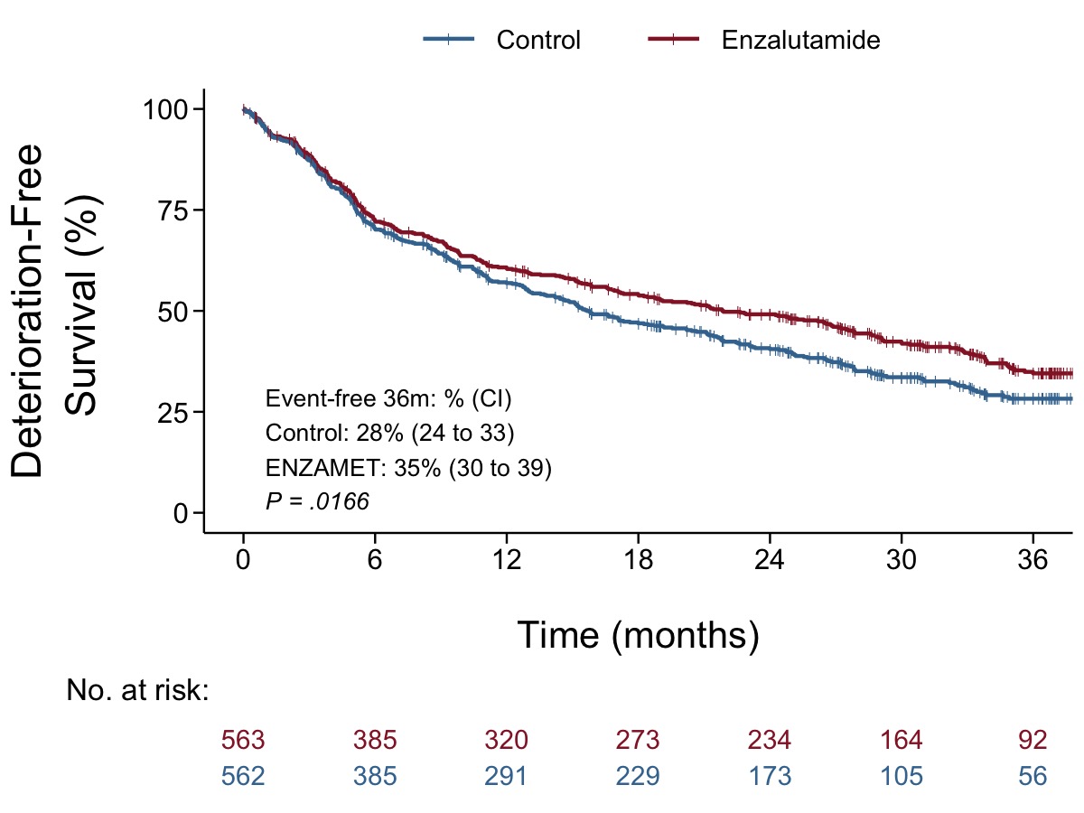
Some personal recommendations:
- It is possible to add annotation as a manual text (totally same with original figure such as 22%, 31%, or P = .0013). However, for the reproducibility, I preferred adding glued text using fabricated data variables.
- The levels of factor in table is reverse order with the legend text. I would prefer presenting control (blue line) first, then experimental (red line).
Or reverse the order of legend text.
Citation
Ali Guner (Jan 31, 2022) Week-3. Retrieved from https://datavizmed.com/blog/2022-01-31-week-3/
@misc{ 2022-week-3,
author = { Ali Guner },
title = { Week-3 },
url = { https://datavizmed.com/blog/2022-01-31-week-3/ },
year = { 2022 }
updated = { Jan 31, 2022 }
}