Posts
This week’s article is from the game-changer FLOT4 trial. I ll replicate a simple but very informative figure.
Selected article:
Title: Histopathological regression after neoadjuvant docetaxel, oxaliplatin, fluorouracil, and leucovorin versus epirubicin, cisplatin, and fluorouracil or capecitabine in patients with resectable gastric or gastro-oesophageal junction adenocarcinoma (FLOT4-AIO): results from the phase 2 part of a multicentre, open-label, randomised phase 2/3 trial
Journal: Lancet Oncology
Authors: Al-Batran SE, Hofheinz RD, Pauligk C et al.
Year: 2016
PMID: 27776843
DOI: 10.1016/S1470-2045(16)30531-9
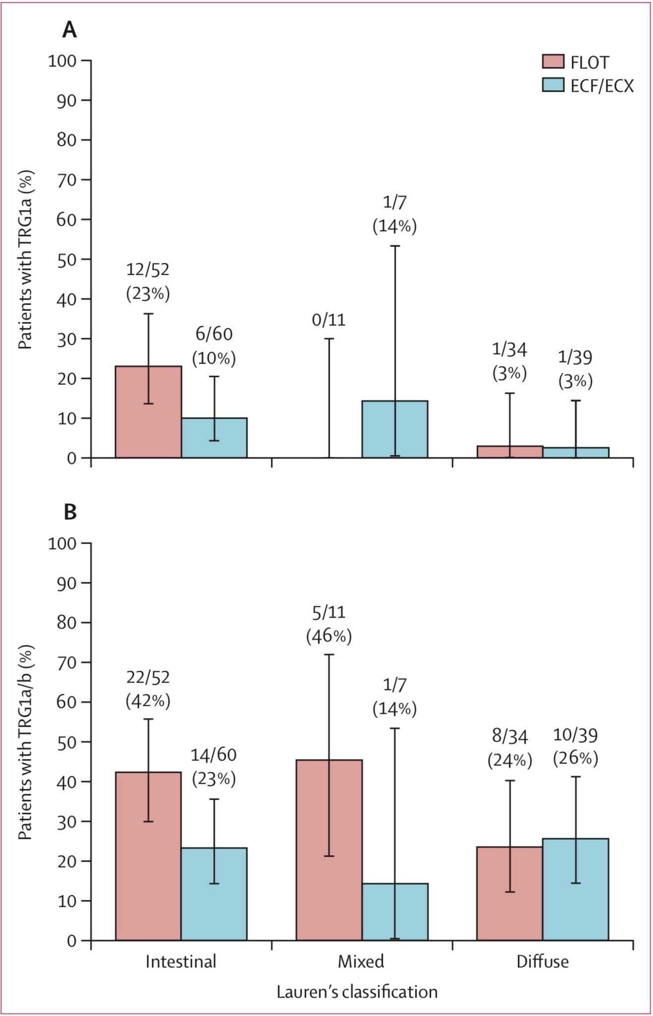
The original figure
Import libraries
library(tidyverse)
library(scales)
library(fabricatr)      # to fabricate fake data
library(glue)           # to prepare label text
library(broom)          # to tidy prop.test()
library(lemon)          # for facet_rep_wrap() function


theme_set(theme_light(base_family = "IBM Plex Sans"))
Prepare fabricated data
# FLOT
set.seed(2022)
FLOT_intestinal <- fabricate(
  N = 52,
  main_group = "FLOT",
  lauren = "intestinal",
  response = c(rep("1a", 12), rep("1b", 10), rep("others", N-22)))

FLOT_mixed <- fabricate(
  N = 11,
  main_group = "FLOT",
  lauren = "mixed",
  response = c(rep("1a", 0), rep("1b", 5), rep("others", N-5)))

FLOT_diffuse <- fabricate(
  N = 34,
  main_group = "FLOT",
  lauren = "diffuse",
  response = c(rep("1a", 1), rep("1b", 7), rep("others", N-8)))


# ECF/ECX
set.seed(2022)
ECF_intestinal <- fabricate(
  N = 60,
  main_group = "ECF/ECX",
  lauren = "intestinal",
  response = c(rep("1a", 6), rep("1b", 8), rep("others", N-14)))

ECF_mixed <- fabricate(
  N = 7,
  main_group = "ECF/ECX",
  lauren = "mixed",
  response = c(rep("1a", 1), rep("1b", 0), rep("others", N-1)))

ECF_diffuse <- fabricate(
  N = 39,
  main_group = "ECF/ECX",
  lauren = "diffuse",
  response = c(rep("1a", 1), rep("1b", 9), rep("others", N-10)))

# Combine datasets
combined_dataset <- bind_rows(
  FLOT_intestinal, FLOT_mixed, FLOT_diffuse,
  ECF_intestinal, ECF_mixed, ECF_diffuse,
) %>%
  mutate(ID = paste0("p_" ,row_number()), .before = "main_group") %>%
  as_tibble()
A part of fake dataset
set.seed(2022)
combined_dataset %>%
  sample_n(10)
## # A tibble: 10 × 4
##    ID    main_group lauren     response
##    <chr> <chr>      <chr>      <chr>
##  1 p_179 ECF/ECX    diffuse    others
##  2 p_55  FLOT       mixed      1b
##  3 p_75  FLOT       diffuse    others
##  4 p_196 ECF/ECX    diffuse    others
##  5 p_6   FLOT       intestinal 1a
##  6 p_191 ECF/ECX    diffuse    others
##  7 p_123 ECF/ECX    intestinal others
##  8 p_14  FLOT       intestinal 1b
##  9 p_7   FLOT       intestinal 1a
## 10 p_93  FLOT       diffuse    others
Possible strategy:
This time, I ll go with faceted figure.
I prefer using geom_col() instead of geom_bar(). Therefore, I ll do some calculations for percentage and CIs.
tidy_data <- combined_dataset %>%
  group_by(main_group, lauren) %>%
  summarise(n = n(),
            n_1a = sum(response == "1a"),
            n_1a1b = sum(response == "1a" | response == "1b")) %>%
  ungroup() %>%
  pivot_longer(cols = c("n_1a", "n_1a1b"),
               names_to = "facet_group",
               values_to = "values") %>%
  rowwise() %>%
  mutate(prop_table = list(tidy(prop.test(values, n, conf.level=0.95)))) %>%
  unnest(prop_table) %>%
  mutate(estimate = estimate * 100,
         conf.low = conf.low * 100,
         conf.high = conf.high * 100) %>%                   # mutate_at() or mutate(across()) is possible.
  select(main_group:estimate, conf.low, conf.high) %>%      # just to simplify the dataset
  mutate_at(c("main_group", "lauren", "facet_group"), factor) %>%
  mutate(main_group = fct_relevel(main_group, c("FLOT")),
         lauren = fct_relevel(lauren, c("intestinal", "mixed", "diffuse"))) %>%
  mutate(label_text = if_else(values == 0, glue("{values}/{n}"), glue("{values}/{n} \n({round(estimate)}%)")))
R codes for the figure
final_replica <- tidy_data %>%
  ggplot(aes(lauren, estimate, fill = main_group)) +
  geom_col(position = "dodge", colour="black", width = .7) +
  geom_errorbar(aes(ymax = conf.high, ymin = conf.low), position = position_dodge(width = .7), width = .15) +
  facet_rep_wrap(~ facet_group, ncol = 1,  strip.position = "left",  labeller = as_labeller(c(n_1a = "Patients with TRG1a (%)", n_1a1b = "Patients with TRG1a/b (%)"))) +
  scale_y_continuous(limits = c(-2, 100), breaks = seq(0,100,10), expand = c(0, 0)) + # -2 was used to add outside ticks
  scale_x_discrete(labels = c("Intestinal", "Mixed",  "Diffuse")) +
  scale_fill_manual(values =  c("#D8A09A", "#9ED0D9")) +
  geom_text(aes(y = conf.high + 8, label = label_text), position = position_dodge(width = .7), size = 4, family = "IBM Plex Sans") +
  geom_hline(yintercept = 0, color = "black", size = .5) +
  labs(y = "",
       x = "Lauren's classification",
       fill = "") +
  theme(plot.margin = unit(c(.5, .5, .5, 0), "cm"),
        plot.background = element_rect(colour = "#BC687F", fill = NA, size = .5),
        strip.placement = "outside",
        strip.background = element_blank(),
        strip.text = element_text(color = "black", size = 11),
        panel.grid = element_blank(),
        panel.border = element_blank(),
        panel.spacing = unit(1, "cm"),
        axis.line = element_line(color = "black"),
        axis.line.x = element_blank(),
        axis.ticks.y = element_line(color = "black", size = .5),
        axis.ticks.length.y = unit(.2, "cm"),
        axis.text.y = element_text(size = 11, color = "black"),
        axis.text.x = element_text(size = 11, color = "black"),
        axis.title.x = element_text(vjust = -1.5),
        legend.position = c(.85, .95),
        legend.text = element_text(size = 12),
        legend.key.height= unit(.4, "cm"),
        legend.spacing.y = unit(.25, "cm"),
        axis.ticks.x = element_blank()) +
  guides(fill = guide_legend(byrow = TRUE)) +
  geom_segment(aes(x = 1.5, xend = 1.5, y = 0, yend = -2)) +
  geom_segment(aes(x = 2.5, xend = 2.5, y = 0, yend = -2)) +
  geom_segment(aes(x = 3.5, xend = 3.5, y = 0, yend = -2))


### SAVE FIGURE
ggsave(final_replica,
       file =file.path ("w7_replica.jpg"),
       dpi = 300,
       width = 6,
       height = 9)
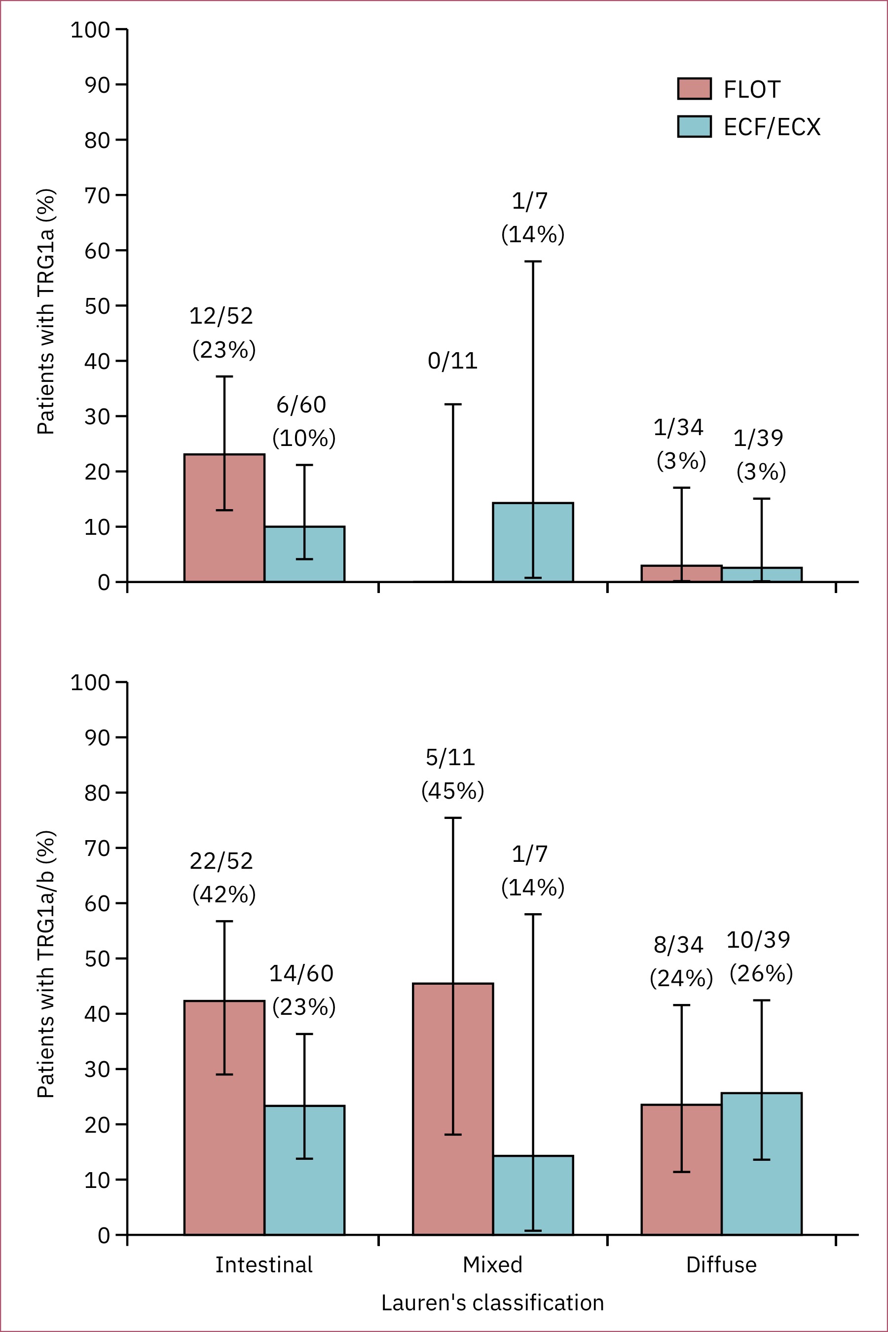
Final replica
Some personal comments:
Citation
Ali Guner (Apr 4, 2022) Week-7. Retrieved from https://datavizmed.com/blog/2022-04-04-week-7/
@misc{ 2022-week-7,
author = { Ali Guner },
title = { Week-7 },
url = { https://datavizmed.com/blog/2022-04-04-week-7/ },
year = { 2022 }
updated = { Apr 4, 2022 }
}